Are you entering the numbers, or is there a formula calculating the number in each cell?
If you are using a formula to create those numbers, the simplest solution would be to wrap the formula in a ROUNDUP statement.
If that would not work, a separate column to round the entered numbers is the only route I can see.
A question: What would 'require editing each time'?
Here's an example whose only required edit prior to a new run is the raw data in column B of of the Data table:
Job 1:

Job 2: No changes to the table except to data in columns A and B
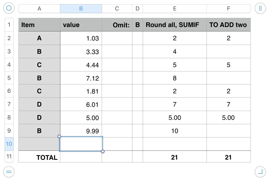
Notes:
Data in columns A and B is entered directly, as is the text in D1, naming the items to be excluded from the totals.
Values in column E are calculated from the value in the same row of column B, using the formula below, entered in E2 and filled down to E10:
IF(B2="","",ROUNDUP(B2,0))
The core formula is shown in bold. It rounds the value in the same row up to the nearest integer. Note that the 5.00 value is not rounded, but retains its two zeroes after the decimal. This can be resolved by setting the data format of cells in this column to 'number' and setting Decimals to 0.
The core formula is wrapped in an IF statement that inserts a null string if the cell on 'this row' of column B is empty.
Row 11, the bottom row of the table, has been 'converted' to a Footer row to omit it from the full column references to columns E and F in the formulas in cells E11 and F11 respectively, and the self-reference error that would occur if the formulas in these cells referenced the cell containing the formula.
The formula in E11is: SUMIF(A,"<>"&D1,E)
The formula tells numbers to SUM all of the (non-header and non-footer) cells in column E where the value in the same row of column A is not the letter in cell D1.
Column F takes a slightly different approach.
Values in this column are calculated using this formula, entered in F2, and filled down to F10:
IF(OR(B2="",A2=D1),"",ROUNDUP(B2,0))
The core formula is the same as in column E, but the IF statement in column F inserts a null string in rows where the cell in column B of 'this row' is empty OR the letter in column A of 'this row' contains the text in cell D1.
Filtering out the values associated with "B" allows a simpler formula in cell F11:
SUM(F)
Either of columns E or F will return the same result. Only one or the other is needed for the table.
EDITING for a new run:
Provided there are enough rows available for the new data set, the only editing involved will be to replace the data in columns A and B with the new data set, and to change the filter out value in D1 if you want to omit a different set of values from the sum.
Longer lists of data will require only adding rows to the bottom of the table (but above the Footer row), and filling the existing formula in row 10 down into th new rows.
Regards,
Barry