SEARCH searching within a string, not a within a range of cells. There are several lookup functions to do lookups on ranges of cells (LOOKUP, XLOOKUP, MATCH, and others) but that is the easy part of the problem. The hard part is you want to find a substring using a longer string. The lookup functions can find the string "Job ABC.pdf" if you search for it, or you can use a substring like "ABC" (along with some wildcards) to find it, but it does not work the other way around. You cannot directly look for "ABC" if you are searching for "Job ABC.pdf". But there is a way to do it.
I am assuming "Job ABC.pdf" was just a simple example and that you cannot easily isolate the "ABC" and search for only that part of the string. If you can, that would likely be far easier than the method I will give below.

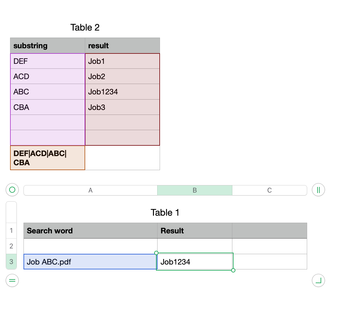
Table 2 is your lookup table. No formulas except in the last row.
Last row is a footer row
Cell A8 (in the footer row) =TEXTJOIN("|",TRUE,A)
Table 1::A3 is your search word
Table 1::B3 =XLOOKUP(IFERROR(REGEX.EXTRACT(LOWER(A3),LOWER(Table 2::A$8)),"Not Found"),Table 2::A,Table 2::B,"Not Found",0)
Let me break down that formula:
- The string in Table 2::A$8 is for use in the REGEX.EXTRACT function. It reads as "DEF or ACD or ABC or...". It is a collection of all the substrings in the column. It becomes the search string, to see if any are in your longer "search word".
- The REGEX.EXTRACT function searches within your search word for any of those substrings. It needs the case to be the same so the search word and the string in Table 2 are first both converted to lowercase. If it finds one, in your search word, the result of REGEX.EXTRACT will be that substring.
- XLOOKUP looks that substring in Table 2::A and returns the result from Table 2::B.
- There are some pieces in the formula to handle cases where there was no match.
Hide the footer row in Table 2 after you have it all working.