Hi Charlene,
Here's a revision that pulls the 20 most recent differentials (and the dates of each of those rounds), extracts the lowest 10 from this list, and calculated the average. The two coloured columns are needed for the calculations, but may be hidden from view.
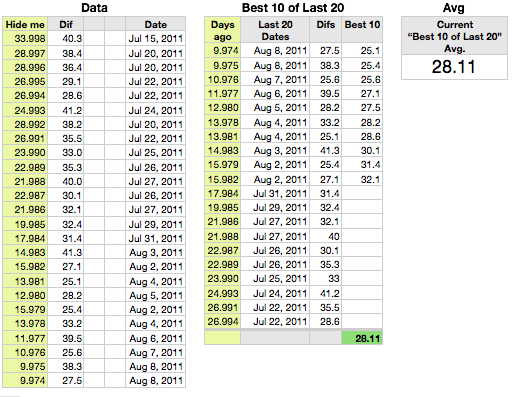
Data is a copy of your table above with an added column on the left to hold values for the VLOOKUP function(s) in the second table. Data in cloumn B is a collection of random values in the range shown in your table. Column E contains a set of random dates (generally increasing, but with some repeats and some out of order). You'll note you had a particularly golf-filled day on July 22.
A2, and filled dow the rest of column A: =DATEDIF(E,TODAY(),"D")-ROW()/1000
This uses DATEDIF to calculate the number of days between Today and the date of the round recorded on this row. The second part (-ROW()/1000) ensures that the value on each row will be unique, necessary if VLOOKUP is to find all three values for July 22 or both values for other days in the list. If more than 400 rounds will be recorded, increase the divisor, 1000, to 10000 or 100000.
The second table, "Best 10 of Last 20" collects the information from the first, and does the calculations. It is a "Sums" table (one Header Row, one Footer Row, no header columns).
A2, and filled down the rest of the column (to A21): =SMALL(Data :: $A,ROW()-1)
This collects the 20 smallest "days ago" numbers from column A of the Data table. Note that the numbers are slightly less than a whole number of days ago, due to the adjustment described above. If you want to display these, you may want to set the cell format to Number, with 0 decimal places.
B2, and filed down the rest of the column (to B21): =VLOOKUP(A,Data :: $A:$E,5,)
C2, and filled down the rest of the column (to C21): =VLOOKUP(A,Data :: $A:$B,2,)
These retrieve the date (column B) and Dif (column C) from the row of Data containing the value in column A.
D2, and filled down ten rows to D11: =SMALL($C,ROW()-1)
D12 - D21 must be empty or contain text. Text and empty cels are ignored by AVERAGE, but any numeric values in these cells will be included in the AVERAGE calculation.
D22 (Row 22 is a Footer Row): =AVERAGE(D)
The average can be calculated here, or the calculation may be done on a separate table.
The third table, Avg., is optional. Itcan be placed onto the same sheet as the Data table to display the average in a convenient place.
A2: =AVERAGE(Best 10 of Last 20 :: D)
Regards,
Barry