Use cells from another table in a Drop Do…

Feb 21, 2013 1:27 AM in response to Elissa C

Hi Elissa,

Here some issues I see with the sample tables provided:

Sale Cover Sheet..the two cells with the input data show"CSI" and "245"

In your previous post, you wrote"

"Let's say there are 4 tables:

1. Input

2. Cover

3. Data

4. Output"

In this post, you show only three.and call the first "Cover Sheet."

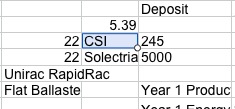
From your description, I'm this table is, for purposes of the VLOOKUP formula, the "Input" table from which the search-for phrase is obtained. For the formula(s), I'll name it Input. The image seems to show only a part of the table, so the cell numbers I've used here are probably incorrect for the actual table.

The selected cell, containing "CSI" is B3. The cell containing "245" is C3. The other cell in that row, A3, also contains data ( "22" ), which also appears on the third table. My assumption is that it is transfered to that table from this one.

Data Sheet (below):

This appears to be the same table as you included in your original post, with one significant change: Where column A of the earlier version contained the manufacturer name, followed by a space and the three digit number from the Watts column, column A of this version contains only the manufacturer name,

To work correctly, the lookup functions need a search-for value that can be found on the lookup table, and that appears only once in the column in which the search is done.

CSI will not work here, as CSI appears twice in column A. Any search for "CSI" will find the one in row 4. (LOOKUP and VLOOKUP start their searches at the bottom of the search column.)

245 (searching column B) would work with this four line sample, as would 240. Each of these numbers appears only once in column B.

But 255 would always find the 255 in B6 (beside LG).

The combined string "CSI 245" would work on the original version of this data table.

On this one, though LOOKUP, using "CSI 245" as its search-for value, and searching column A would always find the first instance of "CSI" in A4. So would VOOKUP if set to look for a close-match. If set to find and exact-match, VLOOKUP would return a 'not found' error.

Step 1: Edit the table below to provide a single match for each search-for value that will be constructed from the values in B3 and C3 of the table above. Column A needs to match column A of the version of this table shown in your original post.

The easiest way to do this is to insert a new column to concatenate (join) the values in columns A and B (and insert a space between the two values) to make a single string that will not be repeated in the table. The search-where column must be the left-most column of the lookup table for VLOOKUP, so to avoid placing it inside the existing table, I would suggest adding a column to the left of column A (click on any cell in column A, press option-left arrow. Columns A and B will be renamed B and C (as will all columns to the right). Vmp will now be in Column I (letter i )

In A3 (to the left of CSI and 245), enter this formula:

=B3&" "&C3

The result displayed will be CSI 245

Fill the formula down the column to the last row of data.

You will now have a search column containing a distinct value on each row, made up of the two values (manufacturer and wattage) you will enter on the input table.

With the new column A added to the Data table, This Lookup table becomes Data::$A:$I

Data Sheet: I will need to populate 4 cells with the data Isc, Imp, Voc and Vmp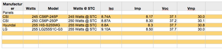

"There are multiple different scenarios where I need to create these Lookups for this spreadsheet and it's definitely complex."

The complexities arise from three sources, from what you've told and showed us so far:

The various Data tables differ in their types of data and in the way this data is arranged.
The output table is arranged differently from the Data table(s) whence it gets its data.
Text is added to some of the data retrieved by VLOOKUP.

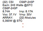
On this table:

A1: (22) CSI — 22 retrieved from Cover table? CSI from Cover table or from Data? (, ) and space entered in formula.

B1: CS6P-245P — retrieved by VLOOKUP from column 4 of Data

A2: "Each: "&245 Watts @ STC — fixed text, concatenated with value from column 5 of the Lookup table.
A3: model number retrieved from B2, or looked up again and retrieved from column 4 of the Lookup table.

A4: 8.74A — value retrieved from column 6 of Data

B4: Imp: 8.17A — value retrieved from column 7 of Data

A5: Voc: 37.1V — value retrieved from column 8 of Data

B5: Vmp: 30V — value retrieved from column 9 of Data

All of the VLOOKUP formulas are very similar. Enter one. Copy its TEXT from the Editor, then paste it into the other cells where VLOOKUP is to be used, and edit the column numbers to match the numbers in the list above.

Syntax for VLOOKUP: =VLOOKUP(search-for,columns-range,return-column,close-match)

In B1, the formula will look like this: =VLOOKUP(Input::B3&" "&Input::C3,Data::$A:$I,4,FALSE)

The returned result will be the model number shown on the sample table above. When that is showing, Click on the cell to select it, then click again to place the insertion point into the cell.

Press command-A to select all of the formula. Copy.

Click Accept to confirm you want to keep this formula in this cell.

In turn, click on each of the cells to receive the formula and Paste. When you have done this, each of these cells should display the model number seen in B1.

For each cell, click twice to enter the editor, then delete the 4 and replace it with the appropriate number from the list above. Click Accept to accept the change, and go on to the next cell.

For cell A2, you will also need to enter the fixed text shown. The formula in this cell will be

="Each: "&VLOOKUP(Input::B3&" "&Input::C3,Data::$A:$I,4,FALSE)

Similar text may need to be added to other cells, depending whether you use the original Data table (which included most of this text in the Data cells, or the newer one from which these labels have been stripped.

Regards,

Barry

Use cells from another table in a Drop Down Menu