Assumed:
Both tables have one header row.
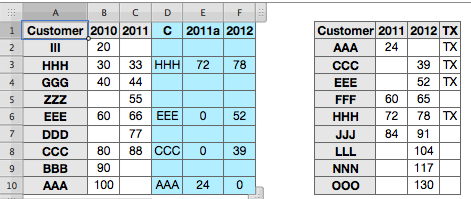
2010 sales on Table 1, 2012 sales on table 2.
Customer names in column A, Sales in columns B and C (both tables)
Ech customer name appears no more than once on each table.
Transfer formulas will copy values from columns A, B and C of Table 2 to columns D, E and F of Table 1
This gives a visual check of matching names in columns A and D of table 1 after the transfer. Column D will be deleted after you are satisfied that the transfer is correct.
You will need to determine how to resolve 2011 sales which may be listed in one, neither or both of columns C and E.
Transfer formulas will be replaced with their results by COPYing the cells in those three columns, then using PASTE VALUES to replace the formulas with the calculated values.
A mark will be placed in Column D of Table 2 to indicate which rows have had their values transferred, and permit easy sorting AFTER using COPPY/PASTE VALUES as above..
Adjust the columns to fit your tables and try this on a COPY of your tables.
Formulas
Table 1:
D2: =IFERROR(VLOOKUP($A,Table 2 :: $A:$C,COLUMN()-3,0),"")
Fill right into E2 and F2, then fill all three down to the bottom row of the table.
Table 2:
D2: =IFERROR(IF(MATCH(A2,Table 1 :: $A,0)>0,"TX",""),"")
Fill down to end of column.
Check that names match in each row of columns A and D.
When satisfied with the transfer, select columns D, E, and F of Table 1, Copy, then go Edit > Paste Values.
Select column D of Table 2. Copy, then go Edit > Paste Values.
Sort Table 2 on column D (the column containing only TX and blank cells).
Select columns A, B and C of the rows that do NOT have TX in column D. Copy.
Click on any cell in Table 1, then use the Row control Handle to add a row to the bottom of Table 1.
Click on the cell in column D of that new row, and Paste.
Select the customer names in the new rows of column D and Copy.
Click on the first new row cell in column A and Paste.
To combine the amounts in columns C and E (2011 sales from each of the two tables), Enter this formula in D2 (replacing the Customer name there):
=C+E
Fill down to the bottom of the column.
With all of column D selected, Copy, then go Edit > Paste values.
Label this column "2011", then selete columns E and C.
Done.
REgards,
Barry