Hi Nick,
Provided all of your names strictly follow the pattern shown in your two examples, the separation is not all that difficult. The process will fail, though, with names such as James Earl Jones.
Ensuring each part begins with a capital adds complexity to the formula. Here, I've done that as a separate step. The formula in columns F, G and H can be combined with those in D, E and F if desired.
Formulas:
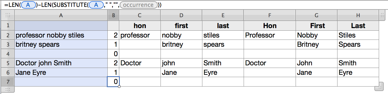
Column B is an auxiliary column. Its results are used in the formulas in the next three columns.
B2, and filled down: =LEN(A)-LEN(SUBSTITUTE(A," ","",))
This counts the number of spaces in the string in Column A.
C2 and filled down: =IF(B<2,"",LEFT(A,FIND(" ",A)-1))
IF returns a null string if the number of spaces in the string in A is less than 2. Otherwise, it passes control to LEFT (and FIND).
Find returns the position of the first space in the string in column A. 1 is subtracted to give the position of the last character to be included in the string placed in this column. LEFT returns the characters the first word.
D2, and filled down: =IF(B<2,LEFT(A,FIND(" ",A)-1),MID(A,FIND(" ",A)+1,FIND(" ",A,FIND(" ",A)+1)-FIND(" ",A)))
IF there are less that two spaces in the string, the 'else' part of the formula above is called to return everything before the first space.
*Note that this will return an error if there are no spaces in the string (eg. Beyoncé, or Sting). See below.
If there are two (or more) spaces, MID returns everything between the first and second space, using the resuts of the first FIND (following MID) to determine where to start, and the results of the second and third FINDs to detrmine how many characters to include.
E2, and filled down: =RIGHT(A,LEN(A)-(B+LEN(C&D))+(B-1))
This returns all characters to the right of the second space in the string in column A
*This will aso return an error if there are no spaces in column A.
Errors:
The two errors above can be trapped using IFERROR.
To do so, enclose each of the formulas with IFERROR, as below:
D2: =IFERROR(IF(B<2,LEFT(A,FIND(" ",A)-1),MID(A,FIND(" ",A)+1,FIND(" ",A,FIND(" ",A)+1)-FIND(" ",A))),"")
E2: =IFERROR(RIGHT(A,LEN(A)-(B+LEN(C&D))+(B-1)),"")
Capitalisation:
Formatting the cells as "Title" displays the initial etter of each word as a capital, but does not change the actual data in the cell. To do that, you'll need to use the UPPER() function.
In the example table, this is done in columns F, G and H, using the data in columns D, E and F respectively.
F2: =IF(LEN(C)>0,UPPER(LEFT(C,1))&RIGHT(C,LEN(C)-1),"")
This formula may be filled right to column H, and filed down each column.
Regards,
Barry