Sorting?

no the formulas I provided take care of that... they must be consistently the relative number of rows and columns away from the name

Here is a screenshot showing the data flow:

find the name in column A of the Pool Standings

retrieve the value from the cell 1 row down in column T

The number in column B is the row the name is in.:

Larry Beamer is in row 3,

Norm Charest is in row 14,

Randy Koons is in row 25,

etc

Dave Lohnman is one of the people whos information is not showing in the column C. Is the spelling the same in both tables?

"Is there a way to add a row of numbers on the left of 1-20 and have that row remain constant?"

I assume you mean a column of numbers placed to the left of the column containing the names in the Ranking table. Numbers 1 to 20 would indicate the rank of each pool member.

Click on any cell in column A, then hover the mouse pointer on the column reference tab. When the triangle appears, click it and choose "Add column before" from the contextual menu.

Check the table to determine if adding this column has broken any of the formulas on the table. If all is OK, continue to the next step. If you see error triangles, or altered results, go Edit > Undo, then skip to ALTERNATE METHOD (below).

Continuing:

Click on the new cell A2, and enter: =ROW()-1

Confirm the entry, then fill the formula down to row 21.

ALTERNATE METHOD:

Add a new Basic table (one header row, no header columns) to the sheet. Delete all but one column, and add or delete rows to make the table 21 rows high.

Click on the new cell A2, and enter: =ROW()-1

Confirm the entry, then fill the formula down to row 21.

Place the new table to the left of the Rankings table. Resize the rows to match rows on the Rankings table.

Regards,

Barry

PS: I've not been following the thread, and haven't examined the suggested formulas to determine the effect of adding a new column to the table. My preference would be to keep all five columns on the same table if that works, and to use the alternate method only if the first breaks the existing formulas.

B

Yes. Add a column and use the formula:

=row()-1

then fill down

This is for

"Is there a way to add a row of numbers on the left of 1-20 and have that row remain constant?"

=row()-1

There will be a similar formula for getting points for getting the $$$

"Is this for the numbering or the $$$ field question?"

The =ROW()-1 formula in my post and in Wayne's will number the rows 1 to 20 (starting at Row 2 and ending at Row 21). That numbering is independent of the values in any of the columns of the Rankings table.

If you want a formula showing the ranking of the $ values, that can be calculated using RANK and the $ values themselves. E is a new column, added to show the $ ranking of the amounts in the W/L column.

A2: =ROW()-1

E2: =RANK(F2,$F,1)

Fill down to row 21.

As written, this shows the rank of the W/L amount within this group of 20 amounts. If you want to show the rank within the full pool, you will need a column (possibly on a separate table) containing the W/L balance for every player in the pool. Replace $F in the RANK formula with a reference to that column.

Regards,

Barry

Hi dtryon,

Here’s a reboot, using Wayne’s two formulas to get to an interim table, listing only:

• the pool member’s names,
• the row that name is on in the table 2013 Pool Standings,
• the name’s current points total from column T,
• and the name’s current dollar total from column S (Week 17)
• plus an index column containing a distinct value, constructed from the points and the row number for each row.

The formulas assume there have been no changes to the positions of names, point totals or W/L totals on your data table from those shown in your screen shots.

Second table (replaces the "Ranking" table in your January 16 screen shot)

The names are entered in column A of a second table, named Aux (short for Auxiliary). The spelling must exactly match that used for each name of the main table (2013 Pool Standings)

R ow 1 is a Header row, containing the following labels:

A1: Name, B1: Row, C1: Points, D1: W/L, E1: Index

B2 contains Wayne’s first formula, with one minor revision: The +1 after MATCH() is omitted.

B2: =IFERROR(MATCH(A2, 2013 Pool Standings::$A,0), "")

Syntax of MATCH:

MATCH(search-for,search-where,match-type)

MATCH gets the value from A2 (“Larry Beamer”), then searches for that value in column A of 2013 Pool Standings, requiring an exact match (specified by the zero)

The search-where list, 2013 Pool Standings::$A, is all of column A, including row 1. Larry’s name is in position 2 of that list, so the formula returns a 2.

If there is no match for search-value, MATCH returns an error. This is caught by IFERROR, and IFERROR returns a null string in place of the error returned by MATCH. (null string: A text string of length zero)

Enter the formula as shown above into Aux::B2, then fill down to B21.

C2 and D2 contain Wayne’s second formula, again with one minor revision:

Each player’s point total is displayed in column T, one row below the row containing his name. But that total, and the W/L total are also displayed in column S, points two rows below the name row and W/L total nine rows below the name row. For consistency in the formulas for retrieving these two values, I’ve chosen to collect both from the same column.

C2: =INDIRECT("'2013 Pool Standings'::S"&B2+2)

D2: =INDIRECT("'2013 Pool Standings'::S"&B2+9)

Syntax for INDIRECT:

INDIRECT(addr-string, addr-style)

The second argument, addr-style, is optional. If set to TRUE or omitted, the address style is A1 (column letter and row number). Set to FALSE, the address style is R1C1, a style that is not supported in Numbers, but is included for ‘compatibility with other appliations.’

INDIRECT constructs a text string from text and values contained in cell(s), and returns the contents of the cell at the address represented by that string.

Both formulas in row 2 reference cell B2, which contains the value 2, the position of Larry B’s name returne by the MATCH formula in B2.

The formula in C2 adds 2 to this value, then concatenates the text string “‘2013 Pool Standings’::S” and the addition result 4 to make the full address:

2013 Pool Standings::S4, pointing to one of the cells containing Larry’s point total.

The formula in D2 uses the same text string and value from B2, but adds 9 to the number in B2 for the full address:

2013 Pool Standings::S11, the cell containing Larry’s current W/L total.

Fill both formulas down their respective columns.

E2 contains a simple formula that adds a tiny amount, dependent on position in the column, to the point value in column C to ensure that each value in the index column is unique within that set. Without this adjustment, only the first-found name associated with repeated scores would be listed.

E2: =C+ROW()/10000

The Aux table will look like the example on the left below. Note that this is a constructed table. I have copied the points and W/L amounts from your January 16 post beginning “Is this what you had in mind…”, and added amounts to the rows not shown in your “Ranking” screen shot. I substituted the easily constucted “Name 1”… names rather than retype your column, and omitted the row numbers in column B as the formulas below (on my Ranking table) do not need them.

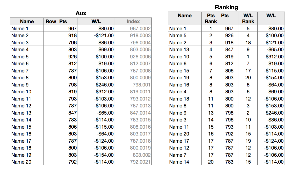
Final table: Ranking

This table, shown to the right above, lists the names, points and W/L amounts in rank order by points, and reports the RANK by points and the RANK by W/L for each name. Note that players with the same total points are assigned the same rank, and the next lower total points is assigned the next available rank.

Example: scores of 10, 10, 9, 8, 8, 8, 3 would be ranked 1, 1, 3, 4, 4, 4, 7.

The table has five columns, Name, Pts Rank, Points, $ Rank, W/L

Labels are placed in Row 1, a Header row.

A2, C2 and E2 contain these similar formulas:

A2: =INDIRECT("Aux::A"&MATCH(LARGE(Aux :: $E,ROW()-1),Aux :: E,0))

C2: =INDIRECT("Aux::C"&MATCH(LARGE(Aux :: $E,ROW()-1),Aux :: E,0))

E2: =INDIRECT("Aux::D"&MATCH(LARGE(Aux :: $E,ROW()-1),Aux :: E,0))

LARGE picks out the index numbers in order, starting with the largest. MATCH returns the position in the list in column E of Aux, and this number is used for the row number of the cell reference constructed in INDIRECT. The three formulas differ only in the column part of that cell reference.

B2 and D2 contain these similar formulas:

B2: =RANK(C,C,)

D2: =RANK(E,E,)

Fill down to the end of their respective columns.

The formula (in B2) returns the rank of the value in C(2) in the list of values in column C. The omitted third argument defaults to “Largest” (967) “is low” ( 1 ).

The ranks in column B are in order because the index column that determines the order in which the Ranking table is loaded is constructed from the Points column on the table AUX.

The ranks in column D are of the money values in column E. These do not appear in order because the money values are ordered by who they belong to, not by their relative value.

Regards,

Barry

PS: Do not sort any of the tables. All sorting is done automatically as data is copied from Aux to Ranking.