Time Sheet Formula Help

Hi,

Have a look at the 'Employee Schedule' template (in your menu File > New and select from the Template Chooser's Business section).

The 'Sign In' table at the bottoms shows one way to set up this type of calculation. In general if you have times in the cells (which are actually date-time values for which you are displaying only the time via Data Format) and you can simply subtract the 'IN' from the 'OUT' to get the duration.

In practice it's not always as simple as subtracting, though. You'll note that the formula in the HOURS column is accounts for that fact that you may have a blank in the IN or the OUT column.

This approach works well unless you have a PM IN followed by an AM OUT time (i.e. "crossing midnight") in which case you'll want to make sure to adjust the date in the OUT column to the following day. If you have a lot of "crossing midnight" shifts, then there are formulas that can deal with that problem automatically.

SG

Hello

If I understand it correctly, you may try something like the following formulae.

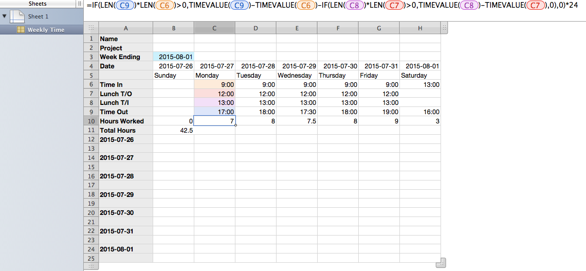
Weekly Time (excerpt) A3 Week Ending A4 Date A5 A6 Time In A7 Lunch T/O A8 Lunch T/I A9 Time Out A10 Hours Worked A11 Total Hours B3 2015-08-01 B4 =C4-1 B5 =DAYNAME(WEEKDAY(B4)) B6 B7 B8 B9 B10 =IF(LEN(B9)*LEN(B6)>0,TIMEVALUE(B9)-TIMEVALUE(B6)-IF(LEN(B8)*LEN(B7)>0,TIMEVALUE(B8)-TIMEVALUE(B7),0),0)*24 B11 =SUM(B10:H10) C3 C4 =D4-1 C5 =DAYNAME(WEEKDAY(C4)) C6 2015-08-01 09:00:00 C7 2015-08-01 12:00:00 C8 2015-08-01 13:00:00 C9 2015-08-01 17:00:00 C10 =IF(LEN(C9)*LEN(C6)>0,TIMEVALUE(C9)-TIMEVALUE(C6)-IF(LEN(C8)*LEN(C7)>0,TIMEVALUE(C8)-TIMEVALUE(C7),0),0)*24 C11 D3 D4 =E4-1 D5 =DAYNAME(WEEKDAY(D4)) D6 2015-08-01 09:00:00 D7 2015-08-01 12:00:00 D8 2015-08-01 13:00:00 D9 2015-08-01 18:00:00 D10 =IF(LEN(D9)*LEN(D6)>0,TIMEVALUE(D9)-TIMEVALUE(D6)-IF(LEN(D8)*LEN(D7)>0,TIMEVALUE(D8)-TIMEVALUE(D7),0),0)*24 D11 E3 E4 =F4-1 E5 =DAYNAME(WEEKDAY(E4)) E6 2015-08-01 09:00:00 E7 2015-08-01 12:00:00 E8 2015-08-01 13:00:00 E9 2015-08-01 17:30:00 E10 =IF(LEN(E9)*LEN(E6)>0,TIMEVALUE(E9)-TIMEVALUE(E6)-IF(LEN(E8)*LEN(E7)>0,TIMEVALUE(E8)-TIMEVALUE(E7),0),0)*24 E11 F3 F4 =G4-1 F5 =DAYNAME(WEEKDAY(F4)) F6 2015-08-01 09:00:00 F7 2015-08-01 12:00:00 F8 2015-08-01 13:00:00 F9 2015-08-01 18:00:00 F10 =IF(LEN(F9)*LEN(F6)>0,TIMEVALUE(F9)-TIMEVALUE(F6)-IF(LEN(F8)*LEN(F7)>0,TIMEVALUE(F8)-TIMEVALUE(F7),0),0)*24 F11 G3 G4 =H4-1 G5 =DAYNAME(WEEKDAY(G4)) G6 2015-08-01 09:00:00 G7 2015-08-01 12:00:00 G8 2015-08-01 13:00:00 G9 2015-08-01 19:00:00 G10 =IF(LEN(G9)*LEN(G6)>0,TIMEVALUE(G9)-TIMEVALUE(G6)-IF(LEN(G8)*LEN(G7)>0,TIMEVALUE(G8)-TIMEVALUE(G7),0),0)*24 G11 H3 H4 =B3 H5 =DAYNAME(WEEKDAY(H4)) H6 2015-08-01 13:00:00 H7 H8 H9 2015-08-01 16:00:00 H10 =IF(LEN(H9)*LEN(H6)>0,TIMEVALUE(H9)-TIMEVALUE(H6)-IF(LEN(H8)*LEN(H7)>0,TIMEVALUE(H8)-TIMEVALUE(H7),0),0)*24 H11

Notes.

Formula in G4 can be filled left.

Formula in B5 can be filled right.

Formula in B10 can be filled right.

Dates in row 5 and day names in row 6 are calculated based upon the date in B3.

Table is built with Numbers v2.

Hope this may help,

H