Alternating Colours in Column

Hi Schrodinger,

Conditional Highlighting may be the solution, but when there is no obvious pattern in the text in column A, I can't find a way to apply it to those cells.

The best I can do is suggest another column that can contain a pattern (even, odd row numbers)

Formula in the new A column (and Fill Down)

=ISEVEN(ROW())

Now Conditional Highlighting to make

• cells with FALSE grey fill and grey text;
• cells with TRUE white text.

I used Custom Style (it has more options). Scroll the Style panel up to see Custom Style.

and use the Rainbow Wheels to choose text and fill colours.

Regards,

Ian.

Hi Schrodinger,

Here'a a solution similar to Ian's, but without the need to add a means of conditional formatting.

I started with a 'standard' table with one header row and one header column, both of which were colour-filled with the default grey fill.

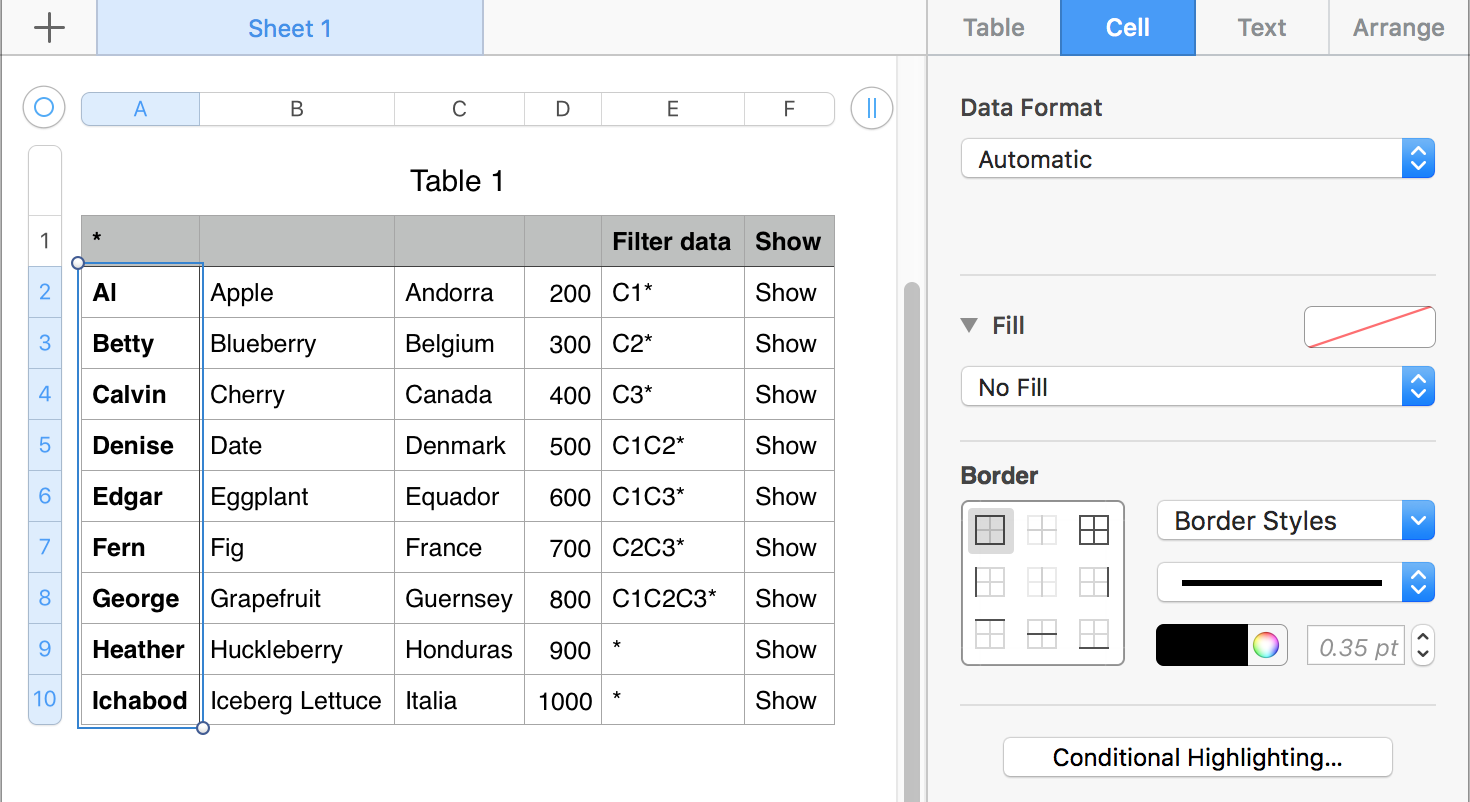
Select all cells in column A except A1, which will remain grey.

In the cell format inspector, choose No fill from the popup menu.

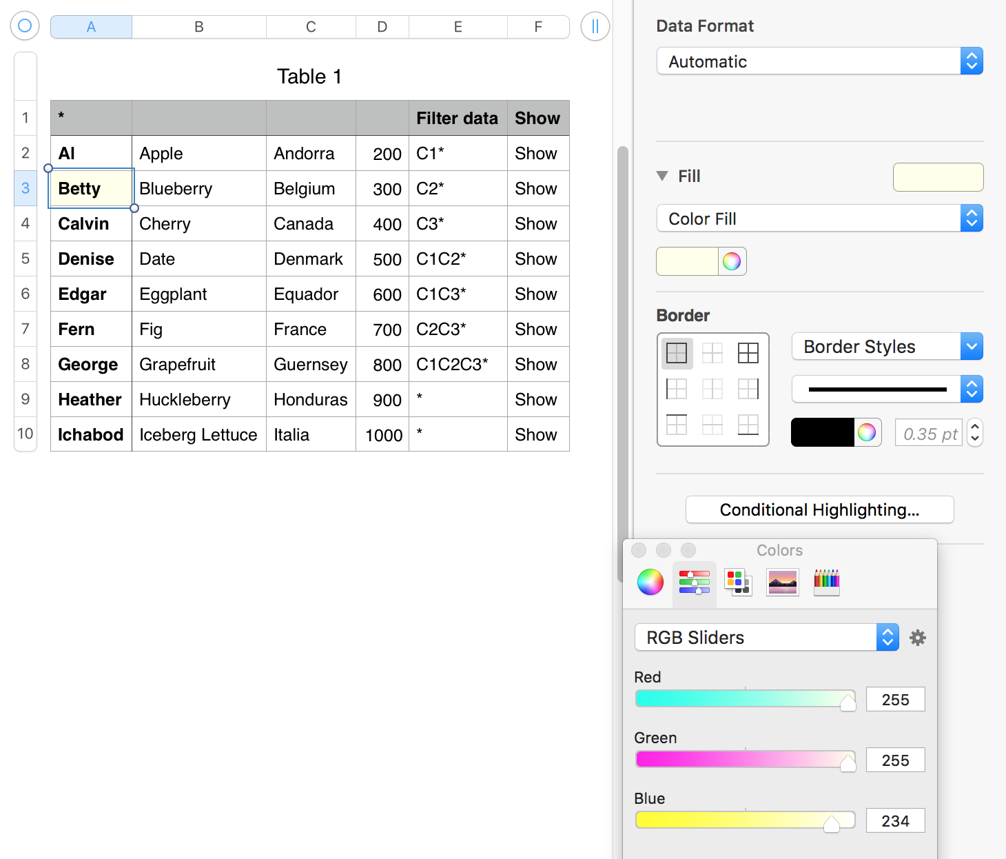
Now select the first cell you want to have a colour fill, choose Color Fill, click the colour wheel and choose an appropriate colour.

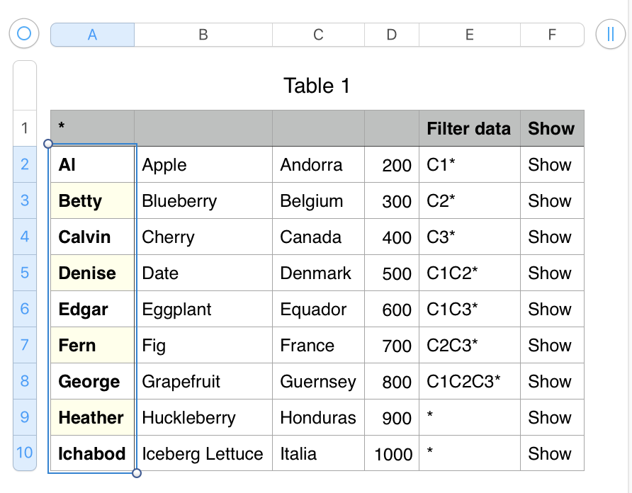
Select the first two non-header row cells in the column and Copy Format (option-command-C).

Select All (non-header row) cells in the column and Paste Format (option-command-V).

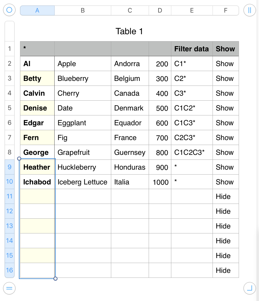
If you later add rows to the table, they will not immediately take on the alternating formats. To apply them, use the last two steps above with this variation:

Select the last two cells in the column on the existing table. Copy Format.

Shift-click on the last cell in the column to extend the selection to the end of the column. Paste Format.

Note: Table shown was originally created to demonstrate use of the Filter to show a selection of rows determine by the the value in A1 being contained in the data in column E. The filter was turned off for this example so the new rows (which contain no data in E) could be shown.

Regards,

Barry