Help in creating a monthly expense report

Hi tkt,

Start by naming your tables. I used short names to keep the formulas short. I'd suggest doing the same while setting them up, then changing the names to what you want once you have the formulas up and running.

If the tables have distinct names, not shared with any other table in the document, then the Sheet names are not needed in the formulas (and Numbers will drop them if you include them).

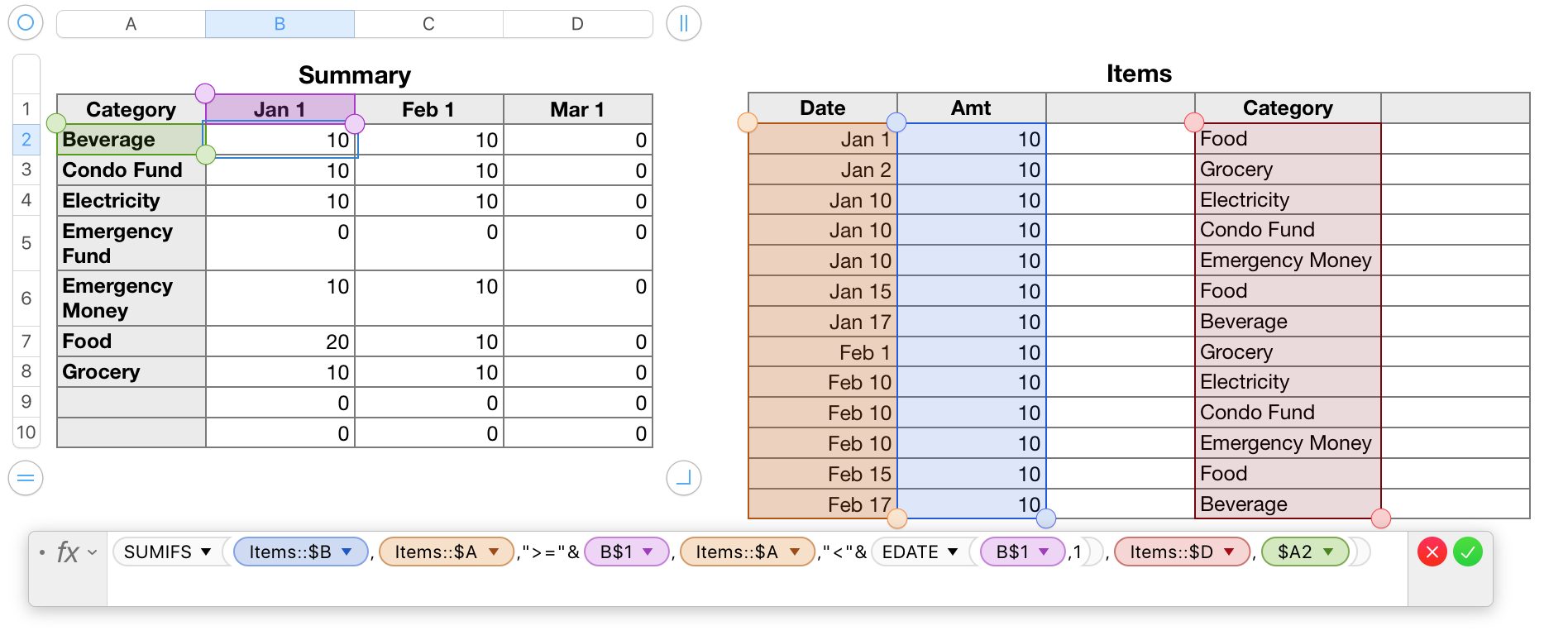
Data is collected on the Items table.

The summary is constructed using the formula shown below the tables (and copied below, with notes).

Items

Dates in column A are entered as the items are recorded. ALL 'dates' in Numbers are Date and time values. If the date is entered as shown, Numbers automatically appends the current year to the Date part, and adds the Time part, set to 00:00:00 (midnight, at the beginning of the day.

Amounts in column B are entered from the keyboard. I left formatting at 'automatic', you may want to use 'number' with 2 decimal places or 'currency' with two decimal places.

Column C represents additional columns used the add details. The column (or columns) does not enter int the formulas.

Category names in column D must match the names in the list of categories in column A of the Summary table.

The easiest way to ensure this is to make the list in Column A of Summary, copy that list, then select cell D2 (one click) and use Edit > Paste and match Style to Paste the list into column D of Items.

Select the cells now containing category names, then set the Data Format for the selected cells to Pop-up menu, and set them to "Start with blank"

Each of those cells then contains a pop-up menu, all with the same choices, and all showing the same value as was originally pasted into that cell.

Set the first one to "none", then use the Fill button (small yellow circle that appears on the bottom edge of the cell when you bring the pointer close to it) the drag a copy into all the cells in that column.

Summary

Column A contains the list of categories to be summarised. As noted above, these must be an exact match to the categories entered in the Items table.

Row 1 contains the first of the month date for each month to be summarised. Each cell contains a full Date and Time value, but is formatted to display only the short monthname and the day nuber (1).

Each of the body cells contains the formula below, entered in B2, then filled to the end of row 2and down to the last row of the table.

SUMIFS(Items::$B,Items::$A,">="&B$1,Items::$A,"<"&EDATE(B$1,1),Items::$D,$A2)

SUMIFS sums the cells in Column B if that match all three of the set conditions:

Items::$A,">="&B$1,                 The date in column A is on or after the date in the header cell of 'this column',

Items::$A,"<"&EDATE(B$1,1),    The date in column A is before the date one month after the date

                                                  in the header cell of 'this column',

Items::$D,$A2                           The category name in column D matches the name in the header cell of 'this row'

Here's a second sample, using the same dates, but with the categories of some expenses changed.

Regards,

Barry

Highly recommend having a look at the Personal Budget template at File > New in your menu. It's a good example of how to do things "the Numbers way."

Here's an expanded version (Dropbox download) the breaks out expenses by month.

The trick is to make sure the spelling of the categories in the Summary table on the first sheet exactly match the categories in the Pop-Up Menu in the Category column in the Transactions table.

SG