Hi J'
Take a look at the Personal Budget template supplied with your copy of Numbers.
The Transactions table there serves the same purpose as your Table 1 above.
The Summary by Category table does in column C, pretty much exactly what you want to do now.
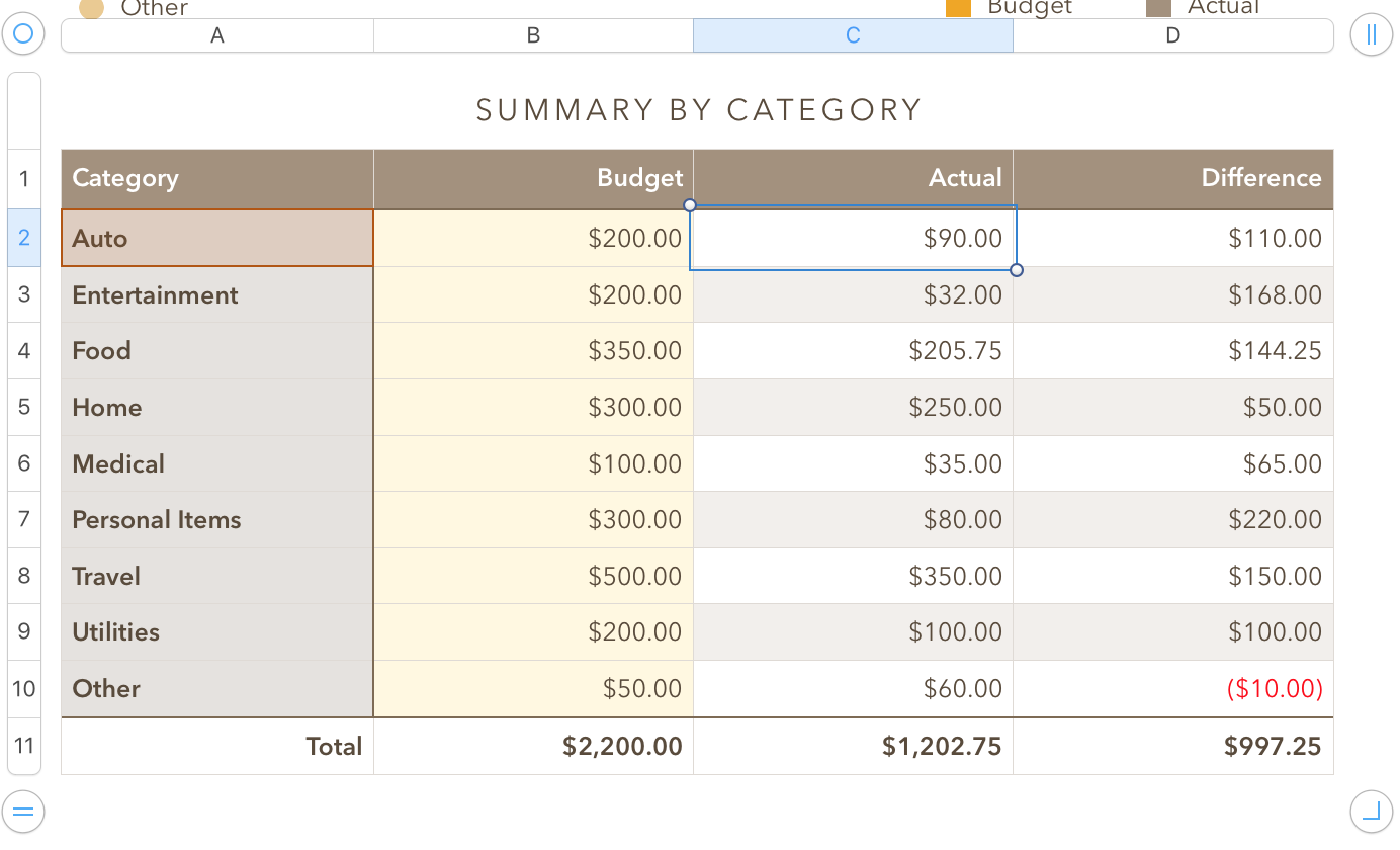
The formula used in column C of this table is:
in C2: SUMIF(Transactions::C,A2,Transactions::$D)
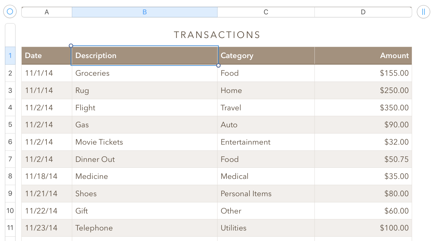
On the Transactions table, column C contains the category label for each transaction, chosen from a pop-up menu in each row.
Column D contains the amount of that transaction.
A2 in the formula refers to cell A2 on 'this table'
The SUMIF formula shown returns the SUM of all values in column D of Transactions where the Category name in column C matches the category name in A2 of this table.
Some notes:
The easiest way to make your pop-up menu cells, if you have not yet started using your data ('transactions') table is to list the categories on the reporting ('summary') table in the order you want to have them in the menu list.
When you've made the list, select all cells with a category name, then click the Format brush, then Cell, choose Pop-up menu from the pop-up currently showing Automatic, then change the pop-up under the menu list from Start with First item to Start with Blank.
Close the inspector, temporarily set the first cell to 'None", making it show a blank, Then copy that cell.
Go to the Category column in your transactions table, make a note of the current category name in each row (if you've already set some), then select the whole column and Paste.
Every cell in the column will now contain the full pop-up menu, and all will be set to None. Use the new pop-up menus to reset the previous labels in the rows that already have entries.
Creating the pop-up cells this way ensures that your category labels on the Summary table match the category labels on the Transaction table.
Getting the labels with a cell reference to column A of the summary table rather than typing each one into a separate formula ensures that you get an exact match for each category.
Regards,
Barry
PS: While Martin is correct about straight and curly quotes not being the same, that issue won't arise here, as MacDonald's is one of the members of the Eating out category on your table, not a category of it's own. Even if it were a category, the use of the same pop-up menu to supply that category name to transactions and to the formula doing the summary ensures an exact match between the category name each time it is used.
B.