how do you populate row cells with fixed data from a drop down menu choice

Hi ladherts,

Here is an example using VLOOKUP to retrieve the information form Data and place it into the correct cell in Nutrition.

Cells A6 to A14 of Nutrition contain copies of the popup menu list shown in this image. As no food has been chosen yet, the cells to the right of column A are all 'blank'.

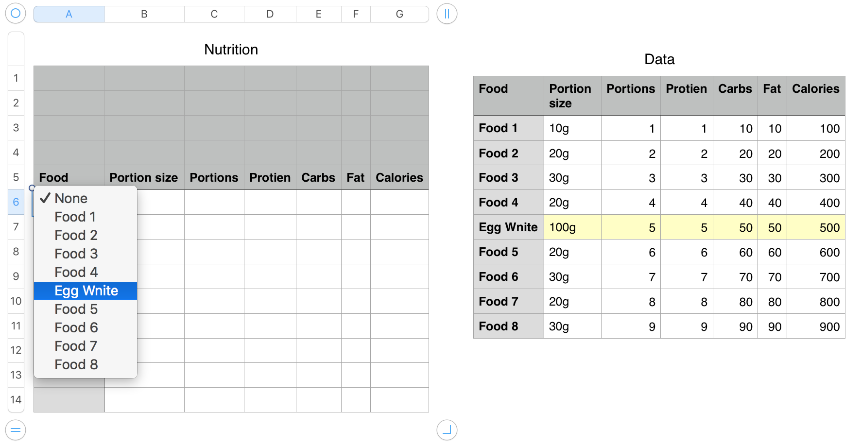
The yellow filled row in Data is coloured manually to make the data in that row more visible for the example. The colour is NOT needed for operation of the document.

In the image below, the user has chosen "Food 8" from the popup menu in cell A6 and "Egg White" from the pop-up menu in cell A9, causing cells in columns B through G of those rows to be filled with the data from the rows of Data containing "Food 8" and "Egg White" in column A.

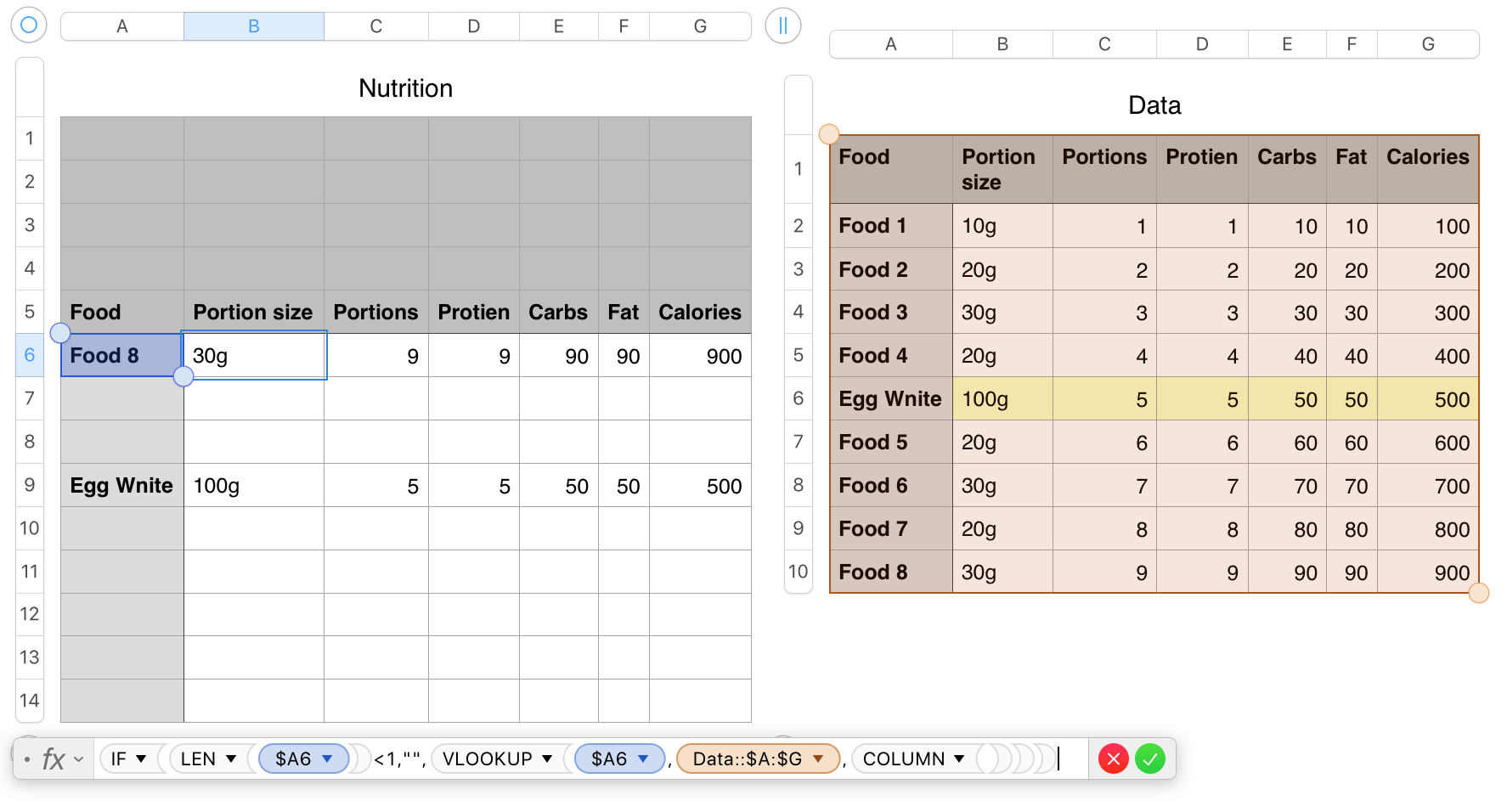
The formula shown below the Nutrition table, is entered as shown in the selected cell (B6), then filled right to G6 and down to row 14,

The formula has two parts—the VLOOKUP part that retrieves the information, wrapped in an IF part that acts as a switch to prevent VLOOKUP from being called before there is a choice made in column A of that row.

As the formula is filled right, the $ operator before each of the column references keeps that part of the reference fixed on the column containing the pop-up menu cells and on the range of columns (A to G) of the Data table.

As the formula is filled down, the number part of the two references to A6 increments to show the same row as is occupied by the row occupied by each copy of the formula.

VLOOKUP always searches in the leftmost column of the lookup table (in this case, column A of Data), then returns the value from the same row of the column specified by the number returned by the COLUMN function.

COLUMN returns the number of the column containing it, which matches the column from which it is to retrieve the data, so column B (2) of Nutrition gets the data from the second column of the lookup table, column B of Data..

Take time to reread as necessary, then enter the formula as shown, into B7 of your Nutrition table, replacing $A6 with $A7 to fit that location.

Regards,

Barry

This is pretty easy to do using a lookup table

For example, if the user sets A7 to 'Egg Whites', a lookup can populate the cells B7-G7 with results from the lookup table.

The lookup table can be hidden or on a different sheet if you prefer.

For example (dummy data, of course)

In this case, the XLOOKUP function takes 4 parameters.

1) The value to lookup (i.e. the option selected from the menu in column A

2) The range in which to search for the value from step 1 - in this case, the $A column in the nutrition table

3) The range in which to find the corresponding value - in this case the corresponding column from the table based on the nutrition data for this column (e.g. 'Portion size', 'portion', etc.)

4) An empty string which is used if the lookup doesn't find a match.

Note this can go a little sideways if the user starts editing values in the main table for whatever reason (basically any edited value will stay even if the food group is changed), but this may not be a problem for you.

Now you can extend this so that the nutrition values are multiplied by the portions - in this way the user can select a food group from the menu, populate the data, and then they can amend 'Portions' to 2 (assuming they were hungry), and the corresponding values would multiple out - that's just normal Numbers functions.

You could use the INDIRECT function, like this:

The first table Targets is the SUMMARY table.

The second table NUTRITION is the table with the Pop-Up menus in the cells of the first column A. Column B, C, ... G contain the INDIRECT function as shown in Formula.

The third table List contains the Food composition data.

All tables might be on the same sheet or on different sheets, depending on how you want to use it.

Paul.

You could add a column Portions (column C, yellow fill) to be used for multiplying the values in the columns D, E, F, G, and H in the table NUTRITION, and fill the formula in D2 right & down, like this:

In the NUTRITION table the Portion column has been moved to the second column B. This column may be hidden when all is working well.

Paul.

In addition I changed the format of the cells in the "Portion Size" column to a Custom Format: "xxx g".

This custom format will add a " g" after the number in the cell but allows you to use the value of the cell for calculations.

Paul.

Here is how I did it:

https://www.dropbox.com/s/m6zslyy2rtwnq9l/Nutrition.numbers?dl=0

It has a table with all the food items for the popup. Whenever I add new items, I finish by selecting all the items in column A, then format as text, sort ascending, followed by formatting as a popup menu. I then copy one of the "---" lines and paste it into the "Blank" sheet/table, all rows other than the two header rows. The "Blank" sheet is my template. To create a recipe or track nutrition for a day, I make a copy of the "Blank" sheet. After making a recipe, you can copy the totals from the top of that table and "paste formula results" into the "food items" table or, for smaller servings of the whole, use a row to divide all those totals by the number of servings it makes then copy/paste formula results.

I included the commonly listed values on nutritional labels and in pretty much the order they appear on the labels. You can search the Internet for "nutrition" and whatever food you want to know about and get a "nutrition label" for it, usually. The nutritional information is serving-size dependent, of course, so it is important to have the serving size be part of the food description. For some things, like canned goods, I typically use the entire can so I adjusted the values for that as my serving size.