"Actually there is a need to yell… because I've tried 3 times to get a simple answer and I get long, drawn out formulas that are completely useless."
Really?
When (and where) did you make these attempts? I don't recall seeing them, nor does a search back through seven pages of questions in the Numbers for Mac community reveal a previous discussion started by "backtopencilandpaper."
What were the "long, drawn out formulas" you received in reply?
Like Badunit, I'm having some difficulty envisioning your table and determining the relationship between the " Amount on 1 end " and the values in the "multiple columns of expense categories". Your question does not appear to include this relationship, so I've ignored "1 end" and considered only the "multiple columns" of categories is the discussion below.
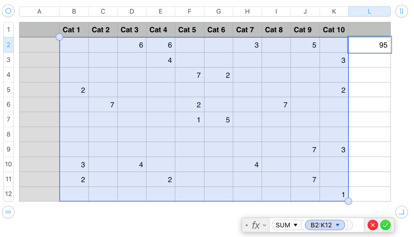
For the exampie, I've used columns B through K to represent the" multiple columns". The table has one Header row (containing the category names, and 11 rows of cells containing the data to be summed.
- - - - - - - - - - - - - - - - - - - - - - - - - - - - - - - - - - - - - - - - - - - - - - - - - - - - - - - - - - - - - - - - - - - - - - - - -
"is there a way to add up all the columns at once"
That can be done with a fairly simple formula, such as the one in L2 of the example below:

But that, according to this, is not the result you are actually looking for:
"Not to get 1 total for all of the columns, but a total for each column."
Assuming you want each of these totals to be displayed in a separate cell, you will need an even simpler formula in each of those cells.
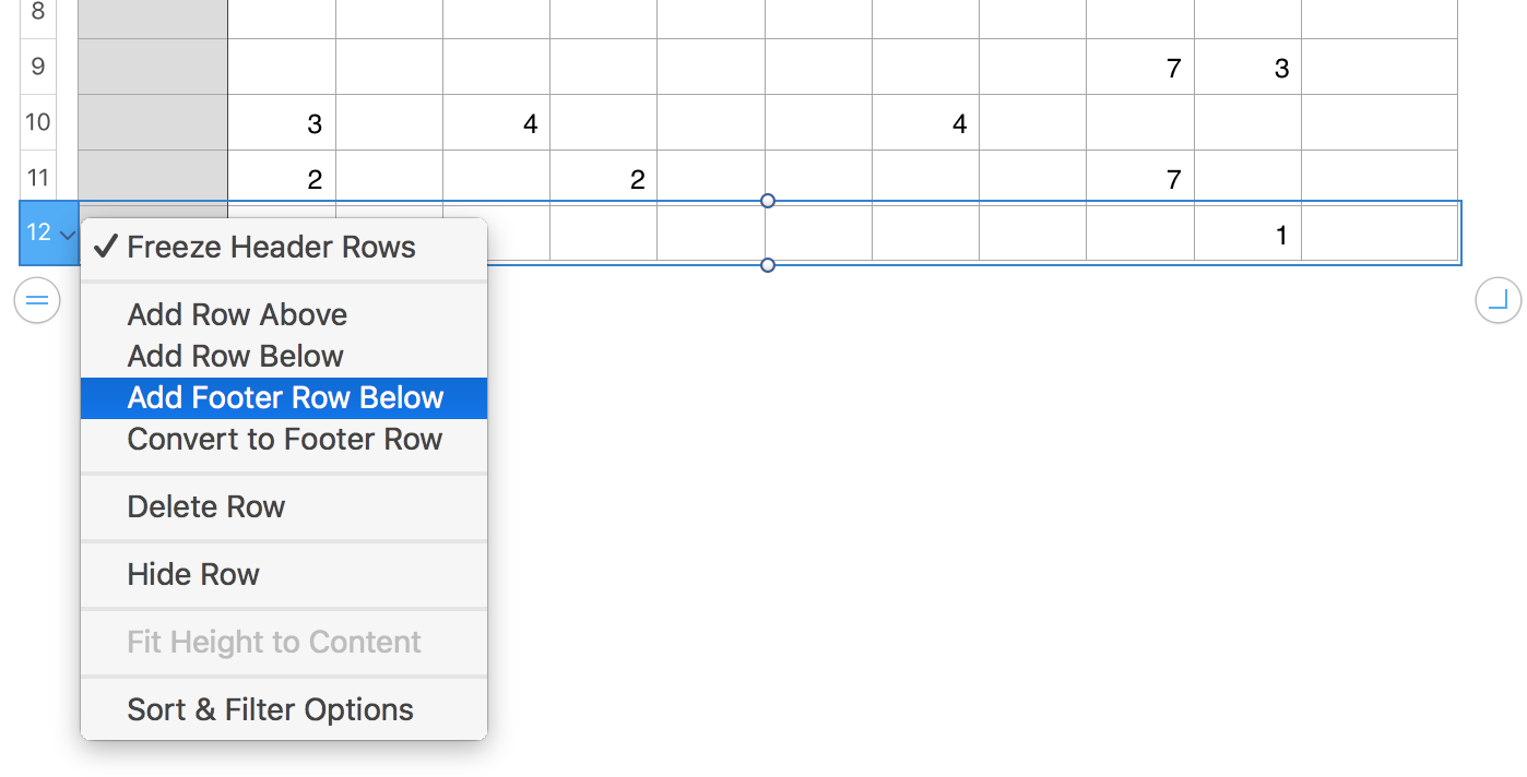
Using the table above. select any cell to activate the table and show the row and column header tabs, then click the tab for the last row (12) to select that row.
Place the mouse pointer in the space between the table and the row 12 tab, and click the 'v' that appears to open the contextual menu shown below. In the menu, choose Add Footer row below (Highlighted in the image below).

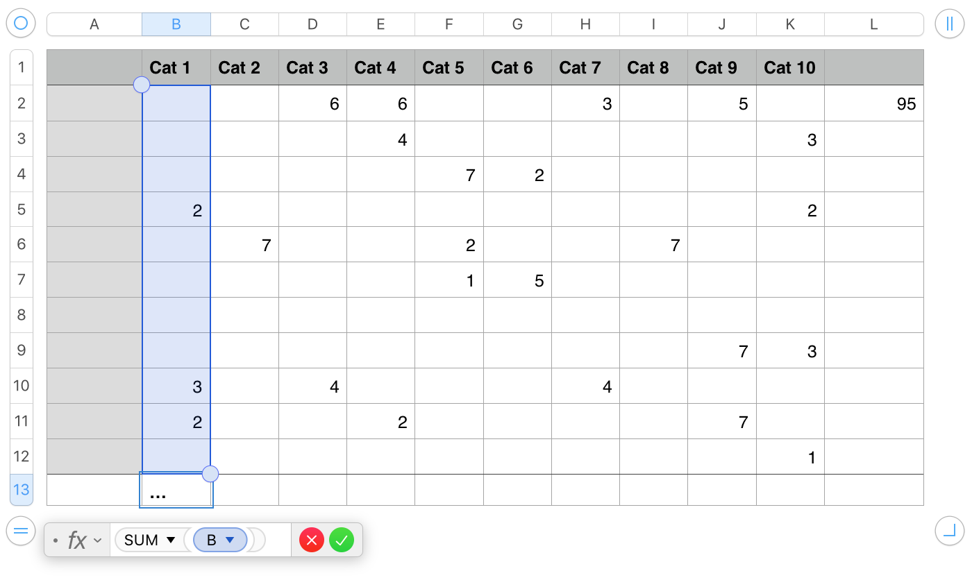
In cell B13, enter this formula: SUM(B)
Then click the green checkmark of the formula editor to confirm the formula and close the editor.

With the formula now showing the sum of values in column B, hover the pointer near the right boundary of cell B13.
A small yellow dot (the Fill Contol) will appear on that boundary.

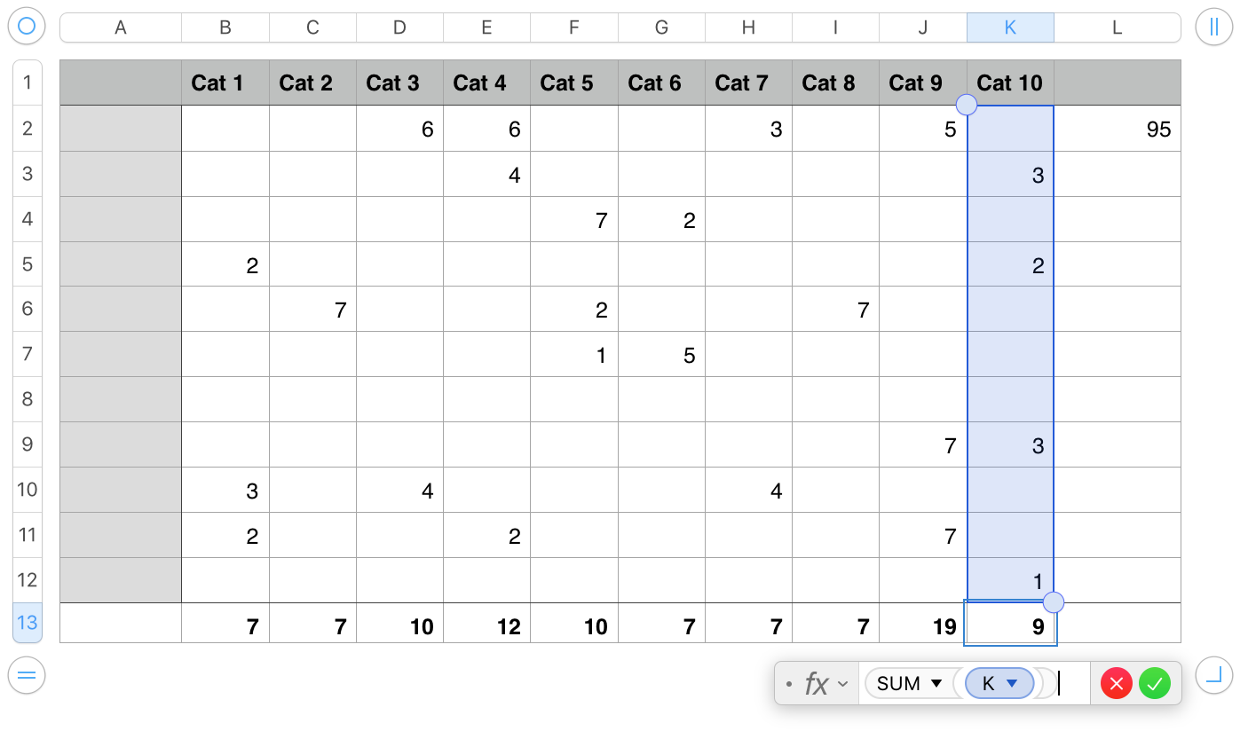
Use the mouse button to grab that control, and drag right to fill the formula into the rest of the cells to K13.
Numbers will automatically increment the column reference to match the column containing each copy of the formula.

Regards,
Barry