More…
Hi C&C
Here is a pair of tables, based on the models in your screenshot. There are three in this 'pair' for reasons discussed below.
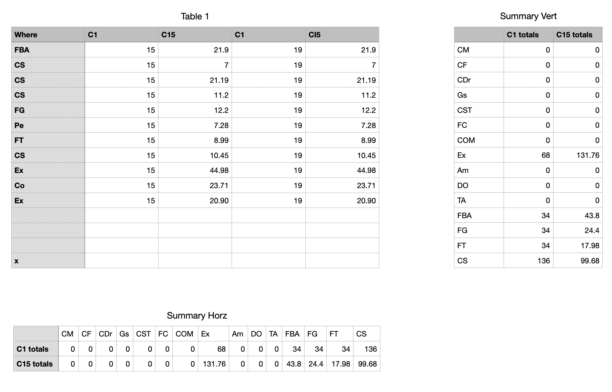
Table 1 is your data table, on which expenditures by C1 are recorded in Columns B and D, expenditures by C15 are recorded in columns C and E, and the location of each expenditure is recorded in column A, using the abbreviations/codes in column 1 and row 1 of the two Summary tables
There are no formulas on this Table.
The table Summary Vert lists codes for all of the locations in column A.
There are two formulas on this table, differing only in the colum letters shown in bold type.
Cell B2: SUMIF(Table 1::A,A2,Table 1::B)+SUMIF(Table 1::A,A2,Table 1::D)
Cell C2: SUMIF(Table 1::A,A2,Table 1::C)+SUMIF(Table 1::A,A2,Table 1::E)
Both formulas are filled down to the last row containing a category code in column A.
The table Summary Horz is a duplicate of Summary Vert.
After making the duplicate, click on a cell to activate the table, then click once on the circle at the intersection of the column and row reference tabs to select the whole table.
Go to the Table menu and choose Transpose rows and columns.
To calculate a grand total of expenditures of each person:
Summary Vert: Add a Footer row to the table. Enter this formula in the Footer cell of column B, then fill it right into column C:
SUM(B)
Summary Horz: Insert a Header column between the current columns A and B. Enter this formula in the Header column cell B2: SUM(2:2)
Fill down to B3.
Regards,
Barry