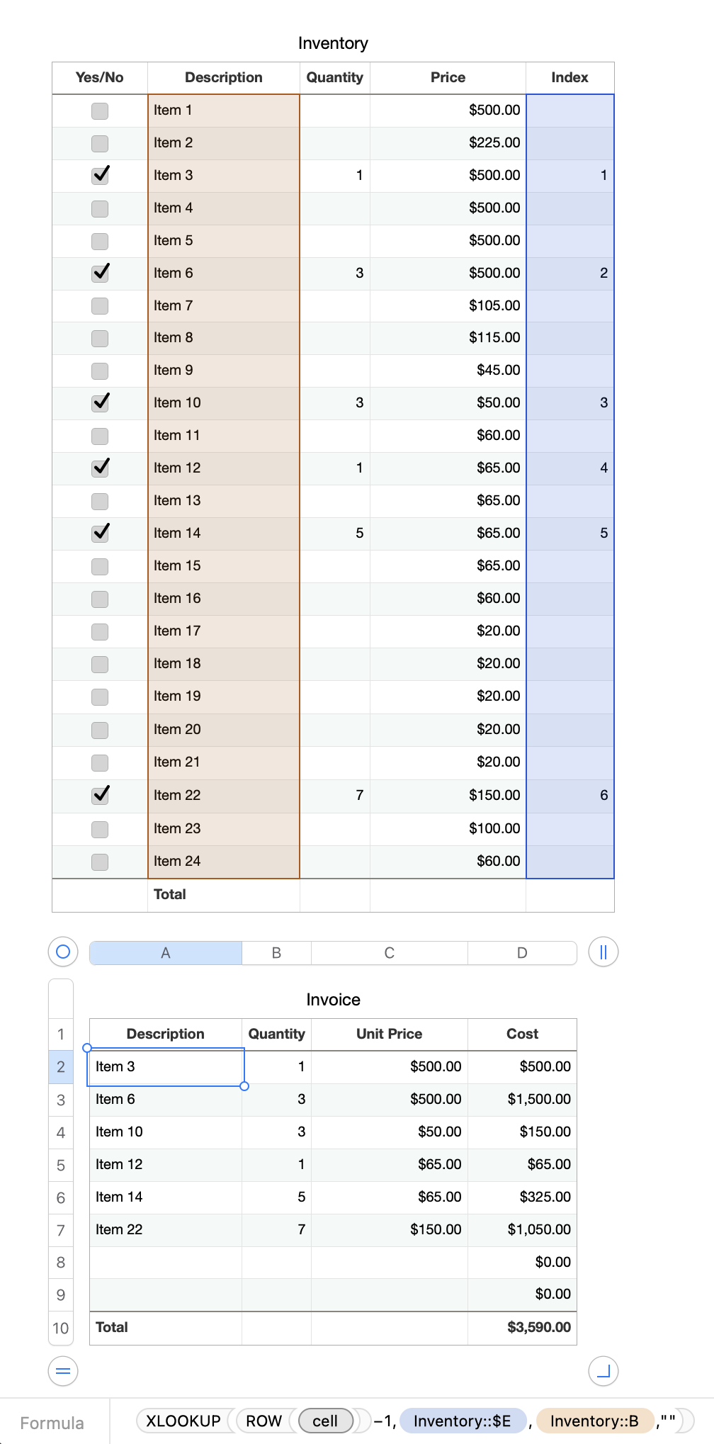
One way is to do something like this:

The formula in E2 (the added "index" column) of the Inventory table is:
=IF(A2,COUNTIF(A$1:A2,TRUE),"")

Fill that down the column, and hide the column if you want.
This increments the index each time it sees a check in column A.
The formula A2 of the 'Invoice' table, filled down is:
=XLOOKUP(ROW()−1,Inventory::$E,Inventory::B,"")
Fill that formula down and right to column C.
(Then you can replace the formula in column B with manually inputted quantities if you want them to be different from the quantities in the Inventory table.)
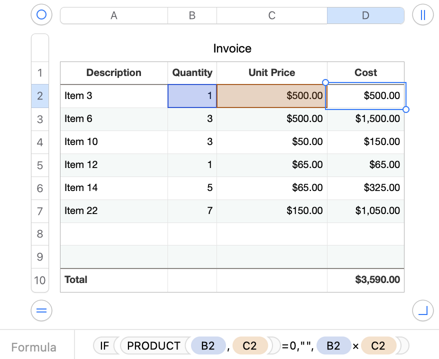
The formula in D2 of the 'Invoice' table, filled down, is:
=PRODUCT(B2:C2) or B2*C2
If you want to keep blank rows at the bottom of your invoice before the total and not show 0s there, then you can use this instead in D2 and fill it down:
=IF(PRODUCT(B2,C2)=0,"",B2*C2)
(Using PRODUCT instead of B2*C2 treats blank cells as 0 instead of throwing an error.)

Remember to use ; instead of , in the formulas if in your region you use , as a decimal separator, i.e. you write 100 dollars as $100,00 instead of $100.00.
SG